This is a blog series around Maester, an AI APIs toolkit project. Check the previous post in the series: Why AI Costs Explode in Production

---

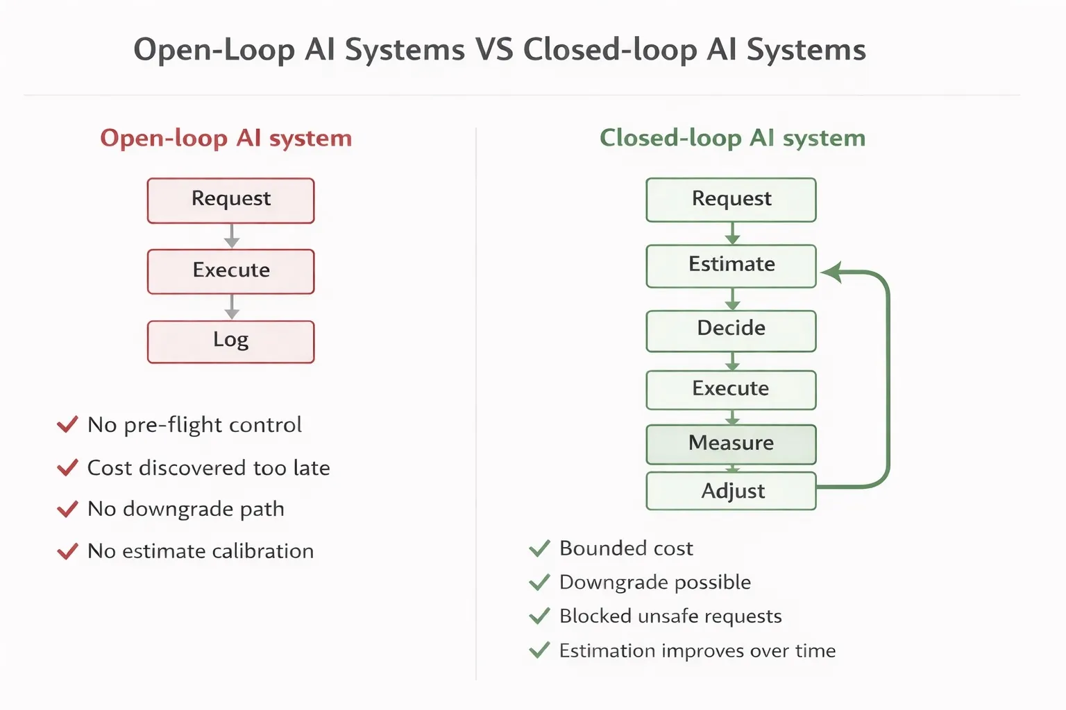
Open-loop vs Closed-loop

When engineers add cost controls to an AI system, the mental model is usually something like this:

observe → decide → act

Watch the spend. If it’s too high, do something. This feels like control. It isn’t.

What you’ve actually built is an open-loop system with a human in the reaction path. By the time a dashboard alert fires, the expensive call has already been made. By the time a human reacts, it’s happened a hundred more times. You’re not controlling the system — you’re auditing it after the fact.

A real control system looks different:

estimate → decide → execute → measure → compare → adjust

This is the closed-loop model from control theory. The distinction isn’t cosmetic. It changes what guarantees the system can make, how it responds to disturbances, and whether it can be analyzed for stability.

---

Why AI Systems Make Control Hard

Before going into the architecture, it’s worth being precise about why controlling AI systems is harder than controlling traditional software.

Traditional systems are deterministic and cost-flat. A database query takes roughly the same time and resources each time. You size it, you monitor it, you scale it. The control problem is well-understood.

LLM systems are none of these things:

They are stochastic. The same input does not produce the same output, and does not consume the same number of tokens. A prompt that generates 200 tokens today might generate 800 tomorrow because the model decided to be more thorough. You cannot predict exact cost from input alone.

They are cost-coupled. Every execution is a direct financial transaction. There is no free retry, no low-cost probe, no “run it first and decide later.” Execution is commitment.

They are partially observable. You cannot inspect internal model state. The only signals available are the inputs you provide, the outputs you receive, and the token counts reported after the fact. The system is a black box with a receipt.

This combination — stochastic outputs, cost-per-execution, limited observability — is exactly the class of problem that control theory was developed to handle. The question is how to formalize it.

---

The Control Loop of AI Systems

Most engineering blog posts skip this step. This is the step that matters most.

A control system cannot be designed without a formal definition of four things: the state, the control inputs, the observations, and the objective function. Without these, what you have is not a control system — it is a collection of heuristics.

State

The system state is the minimal set of variables needed to describe the system’s current condition and predict its future behavior. For an LLM cost control system, the relevant state includes:

• Cumulative spend per scope — the running total spend for a given tenant, user, or workflow. This is the primary variable being regulated.
• Request-level cost — the cost of the current in-flight request, as estimated before execution and measured after.
• Model usage distribution — what proportion of requests are being served by which models. This drives cost variance in multi-model deployments.
• Estimation error — the running delta between predicted cost and actual cost. This is a state variable that most systems ignore, and ignoring it is why estimators degrade silently.

The estimation error deserves special attention. In control theory terms, it is the noise in your measurement channel. If your estimator systematically underestimates by 30%, your controller is making decisions based on a signal that is 30% wrong. The system will appear to be working — requests are being processed, costs are being tracked — but the controller is flying on bad instruments.

Control Inputs

The control inputs are the actuators — the things you can actually change to influence system behavior. For LLM cost control:

• Model selection — routing a request from a capable but expensive model (e.g., GPT-4) to a faster and cheaper one (e.g., GPT-4o-mini). This is the highest-leverage actuator because it affects both cost and latency.
• Token limits — capping the maximum output tokens for a given request. This reduces worst-case cost at the expense of potentially truncated responses.
• Request blocking — rejecting a request entirely when budget is exhausted. This is the hard actuator: zero cost, zero output.
• Routing policies — directing request classes to different execution paths based on cost targets, SLA tiers, or priority levels.

Note that logging is not a control input. This is the most common architectural mistake in LLM cost systems. Recording what happened is observation, not actuation. A system with only logging has no control inputs — it can observe but cannot intervene.

Observations

The observations are what the system can actually measure:

• Actual token count — input and output tokens as reported by the model API after execution.
• Actual cost — derived from token counts and model pricing.
• Latency — execution time per request. Relevant as a secondary objective in latency-constrained deployments.
• Output quality — in most current systems, this is unmeasured. It is the most important future observation: without it, the objective function cannot be fully specified.

The Objective Function

An objective function is a precise mathematical statement of what the system is trying to optimize. Two example formulations:

• Keep system cost within budget constraints

maximize: requests_served
subject to: cumulative_cost ≤ budget_B in window W

• While Maintaining output quality

minimize: E[cost per request]
subject to: quality ≥ Q_min, p99 latency ≤ L_max

The formulation you choose determines everything downstream: which control inputs are used when, how aggressively the system responds to budget pressure, and what tradeoffs are acceptable.

Without an explicit objective function, your control loop is still just storytelling. You have a pipeline with feedback-shaped decorations.

---

Where the System Breaks

Understanding failure modes is what separates a system designer from someone who has assembled components. There are four ways LLM cost control systems fail, and they are not equally obvious.

Failure Mode 1: Open-Loop Systems

The most common production architecture today:

request → execute → log

No pre-execution estimation. No budget check before the call is made. No actuation path. Cost is recorded but never fed back into decision-making.

The consequences are predictable: cost explosions in long-running workflows, no self-correction when usage patterns shift, and complete dependence on human intervention to change behavior. The system has no stability properties because there is no loop.

Failure Mode 2: Delayed Feedback

A step forward — but not enough:

execute → log → dashboard → human reacts

This architecture has feedback, but the feedback delay is measured in minutes to hours. In a high-throughput system, that delay window can contain thousands of requests. By the time the human reacts, the budget has been consumed.

The critical property missing here is pre-execution intervention. A genuine control system must be able to act before the expensive operation executes, not after. This requires moving the decision point upstream.

Failure Mode 3: Unstable Estimators

Even systems with pre-execution budget checks fail if the estimator is unreliable.

If your token estimator has a systematic bias — say, it underestimates by 30% on complex prompts — your controller is making allow/block decisions based on a corrupted signal. Requests that should be blocked get through. Budget is consumed faster than the controller expects. The budget window closes earlier than planned.

More insidiously, estimator accuracy often degrades over time as prompt patterns evolve. An estimator calibrated on one workload can be significantly wrong on another. Without tracking the estimation error as a first-class metric, this drift is invisible until costs blow up.

This failure mode connects directly to system stability: a controller that relies on a biased estimator is not just inaccurate — it is systematically wrong in a consistent direction, which is worse than random noise.

Failure Mode 4: No Actuation Path

The subtlest failure mode. The system observes correctly, estimates correctly, and even makes correct decisions — but has no way to enforce them.

This is the dashboard problem in its purest form. A dashboard can tell you that a request is about to exceed budget. It cannot stop the request. Observation without actuation is not control.

For a system to be a genuine controller, the decision logic must be in the critical path of execution. The request must pass through the controller before it reaches the model. There must be a mechanism to block, downgrade, or reroute — not just record.

---

The Robotic Closed-Loop System

So how would the closed-loop system be built robotically? This was how we built Maester.

The Closed-Loop Architecture

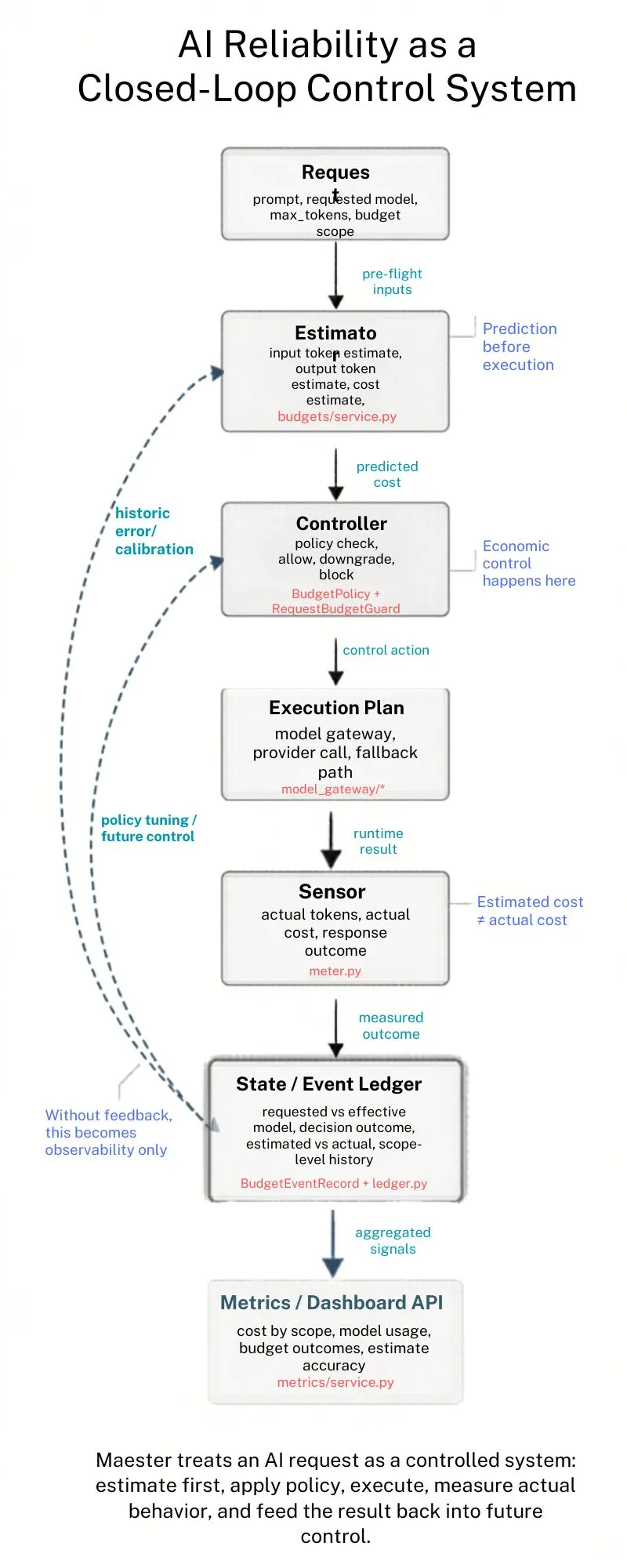
With the formal model defined and the failure modes established, we can now map a concrete implementation. Maester is a budget guard system for LLM workflows.

 estimate → decide → execute → measure → compare → adjust

Step 1: Estimate (The Predictive Model)

Before any request is executed, Maester estimates the token count and associated cost. This pre-execution prediction serves as the setpoint input to the controller.

estimated_tokens = token_estimator.predict(prompt, model)
estimated_cost = pricing.calculate(estimated_tokens, model)

A Control system is only as good as its estimator. Maester treats estimation error as a tracked metric, not a tolerated imprecision. The delta between estimated and actual cost is recorded on every request and can be used to recalibrate the estimator over time.

In control theory terms, this is the reference signal — what the system expects to happen before the plant is engaged.

Step 2: Decide (The Controller)

The budget guard is the controller. It receives the estimated cost, queries the current state (cumulative spend for the relevant scope), and makes a decision:

if estimated_cost + cumulative_spend ≤ budget:
    allow → proceed to execution
elif downgrade_available:
    downgrade → route to cheaper model, re-estimate, re-check
else:
    block → reject request, return budget-exceeded response

This decision logic is the control law. It maps system state and reference signal to a control action. Critically, it executes before the LLM call — which is the property that distinguishes it from a monitoring system.

[image: controller decision flow — allow / downgrade / block paths]

Step 3: Execute (The Plant)

The LLM call is the plant in control theory terms — the physical system being controlled. Maester does not modify the execution itself. It gates and routes it. Once the controller allows a request, execution proceeds normally.

This separation matters architecturally. The controller is decoupled from the execution mechanism, which means it can work across different models, providers, and call patterns without modification.

Step 4: Measure (The Sensor)

After execution, Maester reads the actual token counts and cost from the API response and updates the system state:

actual_tokens = response.usage.total_tokens
actual_cost = pricing.calculate(actual_tokens, model)
state.update(scope, actual_cost)

This is the sensor stage. The measurement closes the loop: actual cost flows back into the state that the controller reads on the next request.

Step 5: Compare (The Error Signal)

The comparator evaluates the estimation error:

estimation_error = actual_cost - estimated_cost

This error signal has two uses. First, it is a diagnostic: large or systematic errors indicate an estimator that needs recalibration. Second, it is a stability signal: if estimation error is large relative to the budget window, the controller is operating on unreliable information.

[image: estimated vs actual cost over time — shows drift and recalibration event]

Step 6: Adjust (The Recalibration Hook)

The final stage is the feedback path back to the estimator. In Maester v0.1, this is a forward hook — the infrastructure is in place for recalibration, with the implementation left for the roadmap.

# Recalibration hook — invoked after each request
estimator.update(
    prompt=request.prompt,
    model=request.model,
    actual_tokens=actual_tokens
)

Even as a future hook, including it in the architecture is the right decision. It makes the system’s evolution path explicit: this is not a monitoring system that might someday gain control features — it is a control system that will tighten its estimation over time.

---

Maester as a Control System

The system guarantees that every component in the loop has a defined role:

Component	Control Theory Role	Maester Implementation
Token/cost estimator	Reference model	Pre-execution token prediction
Budget guard	Controller	Allow / downgrade / block decision
LLM call	Plant	Model API execution
Token count reader	Sensor	Post-execution usage measurement
Error calculator	Comparator	actual - estimated delta
Estimator recalibration	Adjustment	Recalibration hook (roadmap)

---

Tradeoffs

To apply a deterministic control system to a probabilistic system, these are the tradeoffs we should be aware of.

Tradeoff 1: The Stability vs. Responsiveness

Every controller faces a fundamental tradeoff between stability and responsiveness. Maester is no exception.

A controller that is too aggressive — with tight budget windows and aggressive downgrade thresholds — will block or downgrade a high proportion of requests. This is stable in the cost sense but unstable in the quality sense: users experience frequent degradations, workflows fail to complete, and the system becomes brittle.

A controller that is too loose — with wide budget windows and conservative blocking — will absorb cost spikes without response. This preserves quality but sacrifices cost guarantees.

In classical control theory, this is the proportional-integral-derivative (PID) tuning problem. For LLM cost systems, it manifests as the policy configuration problem: how large should the budget window be, how aggressively should the system downgrade, and at what utilization threshold should blocking engage?

There is no universally correct answer. The right configuration depends on the cost sensitivity of the application, the quality requirements of the workload, and the risk tolerance of the operator. What matters is that the system makes this tradeoff explicit and configurable rather than hiding it in hardcoded thresholds.

---

Tradeoff 2: Estimation Error as System Noise

The most sophisticated framing of this architecture treats the estimation error as noise in the control channel.

In a physical control system, sensor noise is a well-understood problem. A noisy position sensor makes a robot’s motion controller less precise. The controller must be designed to be robust to the expected noise level — it cannot assume perfect measurement.

For an LLM cost control system, the analogous problem is this: if your estimator has a variance of ±40% on token counts, then your controller is making decisions based on a signal with ±40% noise. Any budget window tighter than the noise floor is effectively meaningless — the controller cannot distinguish a genuine budget overrun from estimation variance.

estimation_error ~ N(0, σ²)    # in the ideal case of zero-bias estimator

This framing has concrete architectural implications:

• Budget windows should be sized relative to estimator variance, not to absolute cost targets. A 10% budget window with a 30% estimator variance is not a 10% control system — it is an unstable one.
• Estimator confidence should influence controller aggressiveness. When the estimator is uncertain (e.g., on novel prompt patterns), the controller should apply wider safety margins.
• Recalibration should be triggered by noise level, not just by systematic bias. A high-variance estimator is as dangerous as a biased one.

This is the line of thinking that distinguishes a system architect from someone who assembled a pipeline. The question is not just “does the estimator work?” — it is “what are the stability properties of the controller under realistic estimator noise?”

---

Tradeoff 3: Stability vs Responsiveness

The last tradeoff to be aware of is that control systems can become unstable. Control does not guarantee correctness.

Poorly tuned systems can oscillate:

• overly strict policies → excessive downgrades → degraded output quality
• overly loose policies → cost spikes
• repeated adjustments → system instability

Additional instability sources:

• delayed feedback (metrics arrive too late)
• noisy estimations (prediction error)

Designing reliable AI systems is mostly not just about adding controls —
it is about balancing stability vs responsiveness.

---

What This Framing Gives You

The value of applying control theory to AI system reliability is not academic. It is practical.

It makes gaps visible. When you draw the control loop, the missing sensor or the absent actuation path is immediately apparent. You cannot hide “we log this” behind “we handle this.”

It gives you stability vocabulary. You can now ask: “Is this system stable under peak load?” and have a framework to answer it. With an open-loop system, the question is not even well-formed.

It makes the evolution path clear. Every loop component has a known improvement direction: better estimators, tighter controllers, higher-fidelity sensors, adaptive recalibration. The architecture tells you what to build next.

It separates concerns cleanly. The estimator, controller, plant, and sensor are independent components. You can improve the estimator without touching the controller. You can swap the model (plant) without redesigning the sensor.

Most LLM cost systems today are built by adding logging, then adding dashboards, then adding alerts, then adding manual policies — each layer added reactively after a cost incident. The result is an open-loop system dressed as a controller.

Build the loop first. Everything else is calibration.

---

References and Further Reading

• Maester — LLM cost control system: github.com/leiye-07/maester
• Åström, K.J. & Wittenmark, B. — Adaptive Control (2nd ed.) — foundational treatment of controller design under uncertainty
• Doyle, J., Francis, B., Tannenbaum, A. — Feedback Control Theory — formal treatment of stability and robustness
• Sculley et al. — Hidden Technical Debt in Machine Learning Systems (NeurIPS 2015) — the classic argument for treating ML pipelines as engineered systems

Suggested Citation

Lei Ye. Why Your AI System Is Open-Loop. 2026. https://lei-ye.dev/blog/ai-system-control-loop